Spatial transcriptomics deconvolution visualization

We support to visualize the scatterpie chart for any deconvolution or label transferring tools.

Here we will describe how to use SPOTlight and Seurat Label transferring to visualize in stLearn

SPOTlight

You can follow the tutorial of SPOTlight in their git repository: https://github.com/MarcElosua/SPOTlight

After done the tutorial, you can run this R code to get deconvolution_result.csv

# This is R code. You should run this after done SPOTlight tutorial

tmp = as.data.frame(decon_mtrx)
row.names(tmp) <- row.names(brain@meta.data)
write.csv(t(tmp[1:(length(tmp)-1)]),"deconvolution_result.csv")

Note that: - brain is the Seurat object of Spatial Transcriptomics - We save the decon_mtrx to .csv file as the input of our deconvolution visualization function

Seurat label transferring

Seurat provided a vignette about spatial transcriptomics analysis (https://satijalab.org/seurat/v3.2/spatial_vignette.html).

In the section: Integration with single-cell data, you can follow this to do the label transferring.

After that, you can run this code in R to get the deconvolution_result.csv

# This is R code. You should run this after done Integration with single-cell data tutorial

write.csv(predictions.assay@data[-nrow(predictions.assay@data),],"deconvolution_result.csv")

Other software

If you use other software, you should convert the result to this format:

deconvolution_result

	AAACAAGTATCTCCCA-1	AAACACCAATAACTGC-1	AAACAGCTTTCAGAAG-1	AAACAGGGTCTATATT-1	AAACAGTGTTCCTGGG-1	AAACATTTCCCGGATT-1	AAACCGGGTAGGTACC-1	AAACCGTTCGTCCAGG-1	AAACCTAAGCAGCCGG-1	AAACCTCATGAAGTTG-1	...	TTGTGTATGCCACCAA-1	TTGTGTTTCCCGAAAG-1	TTGTTAGCAAATTCGA-1	TTGTTCAGTGTGCTAC-1	TTGTTGGCAATGACTG-1	TTGTTGTGTGTCAAGA-1	TTGTTTCACATCCAGG-1	TTGTTTCATTAGTCTA-1	TTGTTTCCATACAACT-1	TTGTTTGTATTACACG-1
B.cells	0.000000	0.000000	0.000000	0.000000	0.000000	0.000000	0.000000	0.000000	0.000000	0.198548	...	0.420818	0.486748	0.281131	0.000000	0.000000	0.000000	0.498129	0.000000	0.000000	0.626930
BAM	0.000000	0.000000	0.194210	0.000000	0.349818	0.174129	0.128605	0.124109	0.000000	0.000000	...	0.000000	0.000000	0.000000	0.000000	0.193690	0.272291	0.000000	0.000000	0.000000	0.177772
cDC1	0.000000	0.000000	0.000000	0.000000	0.000000	0.000000	0.000000	0.000000	0.000000	0.000000	...	0.000000	0.000000	0.000000	0.000000	0.000000	0.000000	0.149757	0.000000	0.000000	0.000000
cDC2	0.000000	0.000000	0.000000	0.000000	0.287142	0.000000	0.000000	0.000000	0.000000	0.000000	...	0.000000	0.000000	0.000000	0.000000	0.000000	0.000000	0.186463	0.000000	0.000000	0.000000
ILC	0.247162	0.000000	0.000000	0.000000	0.000000	0.000000	0.147220	0.000000	0.000000	0.000000	...	0.000000	0.000000	0.192057	0.000000	0.000000	0.000000	0.000000	0.000000	0.000000	0.000000
Microglia	0.220380	0.166595	0.000000	0.181610	0.000000	0.000000	0.198072	0.000000	0.166483	0.172001	...	0.320737	0.314146	0.000000	0.187380	0.234365	0.000000	0.165652	0.164594	0.229121	0.000000
migDC	0.000000	0.000000	0.000000	0.000000	0.000000	0.000000	0.000000	0.126951	0.000000	0.000000	...	0.000000	0.199107	0.000000	0.000000	0.000000	0.000000	0.000000	0.000000	0.000000	0.000000
Monocytes.Mdc	0.000000	0.000000	0.000000	0.000000	0.000000	0.000000	0.000000	0.000000	0.000000	0.000000	...	0.000000	0.000000	0.000000	0.000000	0.000000	0.000000	0.000000	0.000000	0.000000	0.000000
Neutrophils	0.207182	0.000000	0.182595	0.151981	0.000000	0.000000	0.000000	0.149797	0.349811	0.000000	...	0.000000	0.000000	0.000000	0.000000	0.000000	0.000000	0.000000	0.000000	0.192915	0.195298
NK.cells	0.000000	0.000000	0.177223	0.000000	0.000000	0.000000	0.000000	0.000000	0.000000	0.000000	...	0.000000	0.000000	0.000000	0.000000	0.219932	0.000000	0.000000	0.000000	0.000000	0.000000
Others	0.325277	0.441767	0.270445	0.344442	0.000000	0.484492	0.222825	0.324590	0.000000	0.410401	...	0.258446	0.000000	0.253745	0.403855	0.193312	0.344915	0.000000	0.319064	0.267189	0.000000
pDC	0.000000	0.000000	0.000000	0.152278	0.000000	0.000000	0.000000	0.000000	0.293502	0.000000	...	0.000000	0.000000	0.000000	0.224080	0.000000	0.000000	0.000000	0.187533	0.143427	0.000000
T.NKT.cells	0.000000	0.212961	0.000000	0.169689	0.157046	0.167671	0.160222	0.146710	0.190204	0.000000	...	0.000000	0.000000	0.000000	0.000000	0.000000	0.382794	0.000000	0.328808	0.000000	0.000000
yd.T.cells	0.000000	0.178677	0.175527	0.000000	0.205995	0.173708	0.143056	0.127842	0.000000	0.219050	...	0.000000	0.000000	0.273067	0.184685	0.158700	0.000000	0.000000	0.000000	0.167349	0.000000

14 rows × 2968 columns

Note: - Columns are spot barcode - Rows are labels - Values are the proportion or probability value

stLearn deconvolution visualization

Running the basic analysis step of stLearn

import stlearn as st

data = st.Read10X(path="BRAIN_PATH")
data.var_names_make_unique()
st.pp.filter_genes(data,min_cells=3)
st.pp.normalize_total(data)
st.pp.log1p(data)
st.pp.scale(data)

Variable names are not unique. To make them unique, call `.var_names_make_unique`.
Variable names are not unique. To make them unique, call `.var_names_make_unique`.

Normalization step is finished in adata.X
Log transformation step is finished in adata.X
Scale step is finished in adata.X

st.em.run_pca(data,n_comps=10,random_state=0)
st.pp.neighbors(data,n_neighbors=15,use_rep='X_pca',random_state=0)
st.tl.clustering.louvain(data,random_state=0)
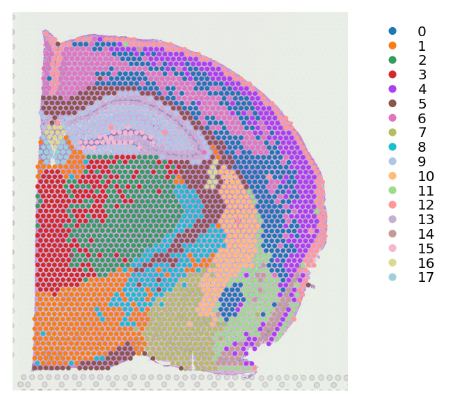
st.pl.cluster_plot(data,use_label="louvain",image_alpha=1,size=7)

PCA is done! Generated in adata.obsm['X_pca'], adata.uns['pca'] and adata.varm['PCs']
Created k-Nearest-Neighbor graph in adata.uns['neighbors']
Applying Louvain clustering ...
Louvain clustering is done! The labels are stored in adata.obs['louvain']

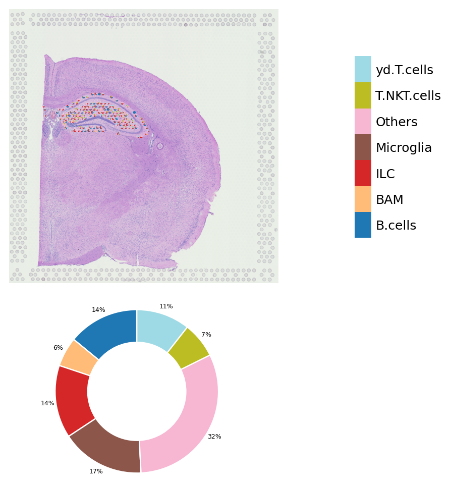
Add annotation from other software and visualize it into a scatter pie plot with donut chart

st.add.add_deconvolution(data,annotation_path="deconvolution_result.csv")

The annotation is added to adata.obs['louvain_anno']

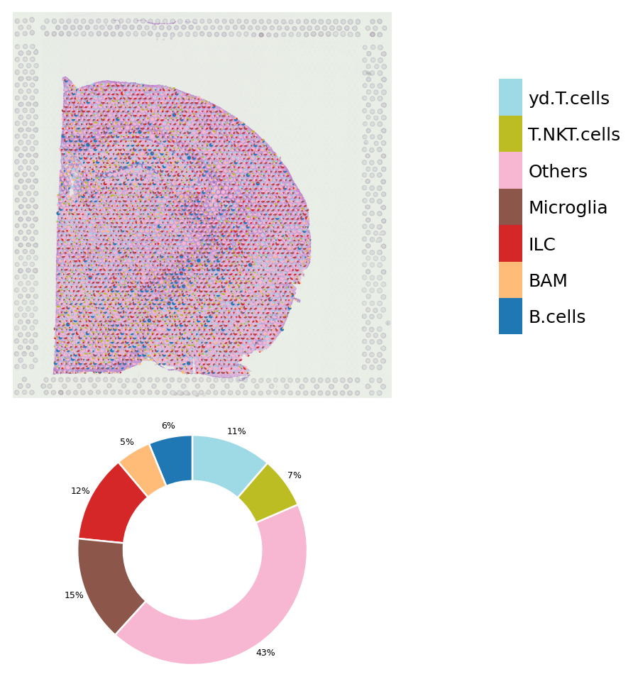
We also provide a threshold parameter that do the filtering based on quantile. The objective is removing the noise labels.

st.pl.deconvolution_plot(data,threshold=0.5)

st.pl.deconvolution_plot(data,threshold=0.0)

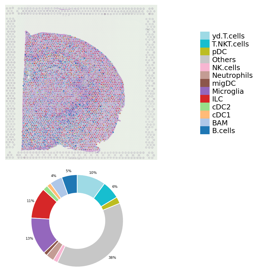
You also can examine the proportion of cell types in each cluster

deconvolution_plot(data,cluster=9)