Xenium stLearn CCI Gridding tutorial
This tutorial runs through stLearn CCI analysis on extremely large data, containing >166,000 single cells with gene expression measured in space.
To increase computation speed, we grid the cells and perform stLearn CCI analysis while taking into account the proportion of different cell types detected per grid.
Environment setup
[ ]:
import pandas as pd
import numpy as np

import stlearn as st
import scanpy as sc

import warnings
warnings.filterwarnings("ignore")
Loading the data
For this tutorial purpose, we don’t perform the clustering. Please run the clustering method with the clustering tutorial or a part of spatial trajectory inference tutorial.
[6]:
adata = sc.read_h5ad('xenium_louvain.h5ad')
[7]:
adata.X = adata.layers['raw_count'].copy()
adata.X
[7]:
array([[0., 3., 1., ..., 0., 6., 1.],
       [0., 0., 0., ..., 0., 1., 0.],
       [0., 0., 0., ..., 0., 0., 0.],
       ...,
       [4., 1., 6., ..., 0., 0., 3.],
       [1., 0., 0., ..., 0., 0., 0.],
       [4., 1., 4., ..., 0., 0., 0.]], dtype=float32)
[8]:
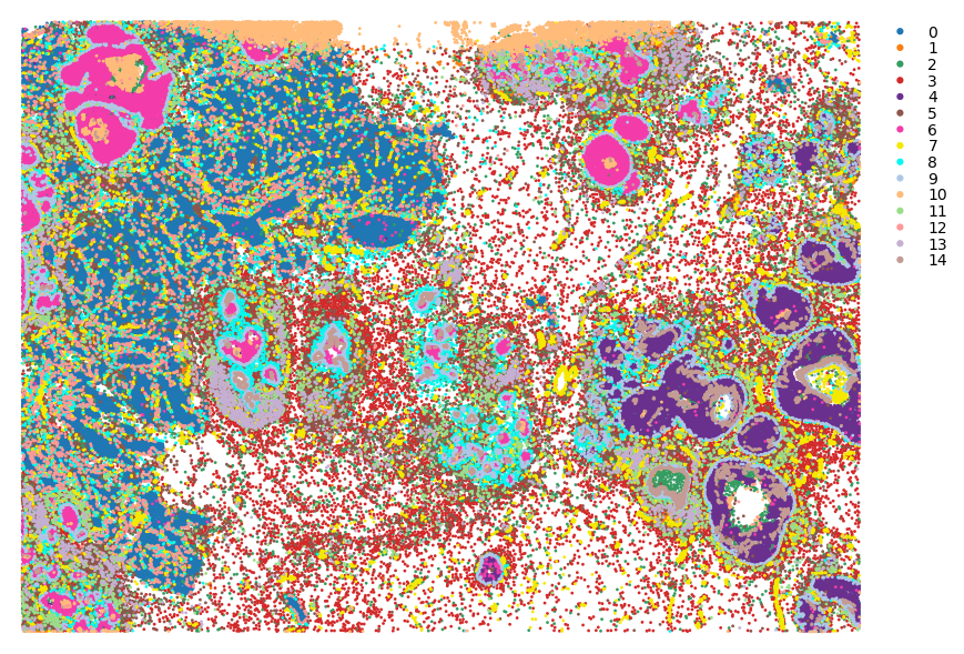
st.pl.cluster_plot(adata, use_label="louvain", image_alpha=0, size=4, figsize=(10, 10))
Note on normalisation
No log1p or shrinking to make genes of similar expression range. In our case, for calling hotspots, we want genes to be more separate, since we select background genes with similar expression levels to detect hotspots.
[9]:
#### Normalize total...
st.pp.normalize_total(adata)
adata.X
Normalization step is finished in adata.X
[9]:
array([[0.        , 3.2922077 , 1.0974026 , ..., 0.        , 6.5844154 ,
        1.0974026 ],
       [0.        , 0.        , 0.        , ..., 0.        , 2.640625  ,
        0.        ],
       [0.        , 0.        , 0.        , ..., 0.        , 0.        ,
        0.        ],
       ...,
       [1.6650246 , 0.41625616, 2.497537  , ..., 0.        , 0.        ,
        1.2487684 ],
       [1.4083333 , 0.        , 0.        , ..., 0.        , 0.        ,
        0.        ],
       [1.7201018 , 0.43002546, 1.7201018 , ..., 0.        , 0.        ,
        0.        ]], dtype=float32)
Gridding
Now performing the gridding. The resolution chosen here may effect the results. The higher resolution, the better this represents the single cell data but the longer the computation takes.
To summarise the gene expression across cells in a grid, we sum the library size normalised gene expression. Summing allows for representing the fact there are multiple cells in a given spot.
[10]:
### Calculating the number of grid spots we will generate
n_ = 125
print(f'{n_} by {n_} has this many spots:\n', n_*n_)
125 by 125 has this many spots:
 15625
By providing ‘use_label’ to the function below, the cell type information is saved as deconvolution information per spot, and also the dominant cell annotation. That way we can perform stLearn CCI with the cell type information!
[11]:
### Gridding.
grid = st.tl.cci.grid(adata, n_row=n_, n_col=n_, use_label = 'louvain')
print( grid.shape ) # Slightly less than the above calculation, since we filter out spots with 0 cells.
Gridding...
(14521, 313)
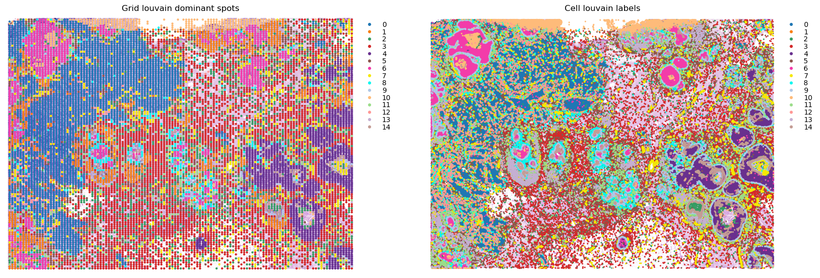
Checking the gridding
Comparing the gridded data to the original, to make sure it makes sense.
It’s recommend to visualise the dominant cell types per spot, in order to gauge whether the tissue structure is adequately maintained after gridding (i.e. to make sure it is not too low resolution!).
[16]:
import matplotlib.pyplot as plt
fig, axes = plt.subplots(ncols=2, figsize=(20,8))
st.pl.cluster_plot(grid, use_label='louvain', size=10, ax=axes[0], show_plot=False)
st.pl.cluster_plot(adata, use_label='louvain', ax=axes[1], show_plot=False)
axes[0].set_title(f'Grid louvain dominant spots')
axes[1].set_title(f'Cell louvain labels')
plt.show()
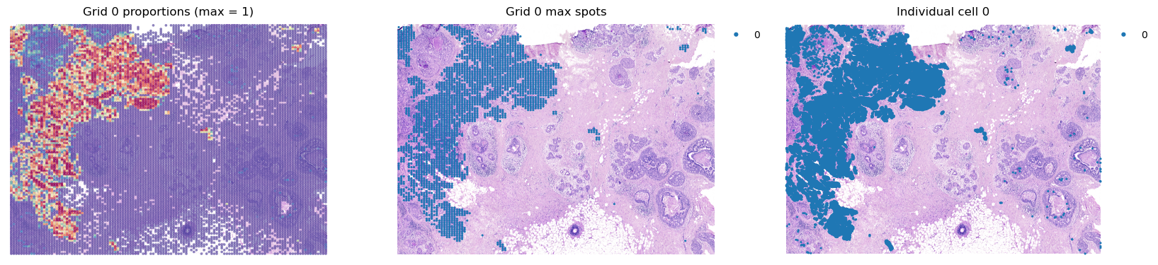
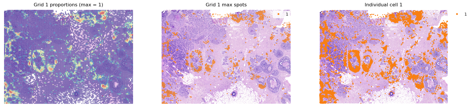
[24]:
groups = list(grid.obs['louvain'].cat.categories)
for group in groups[0:2]:
    fig, axes = plt.subplots(ncols=3, figsize=(20,8))
    group_props = grid.uns['louvain'][group].values
    grid.obs['group'] = group_props
    st.pl.feat_plot(grid, feature='group', ax=axes[0], show_plot=False, vmax=1, show_color_bar=False)
    st.pl.cluster_plot(grid, use_label='louvain', list_clusters=[group], ax=axes[1], show_plot=False)
    st.pl.cluster_plot(adata, use_label='louvain', list_clusters=[group], ax=axes[2], show_plot=False)
    axes[0].set_title(f'Grid {group} proportions (max = 1)')
    axes[1].set_title(f'Grid {group} max spots')
    axes[2].set_title(f'Individual cell {group}')
    plt.show()
[28]:
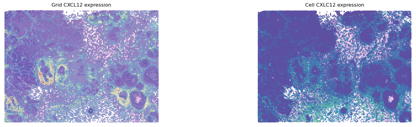
fig, axes = plt.subplots(ncols=2, figsize=(20,5))
st.pl.gene_plot(grid, gene_symbols='CXCL12', ax=axes[0],show_color_bar=False,show_plot=False)
st.pl.gene_plot(adata, gene_symbols='CXCL12', ax=axes[1], show_color_bar=False, show_plot=False,vmax=80)
axes[0].set_title(f'Grid CXCL12 expression')
axes[1].set_title(f'Cell CXLC12 expression')
plt.show()
LR Permutation Test
Running the LR permutation test, to determine regions of high LR co-expression.
[29]:
# Loading the LR databases available within stlearn (from NATMI)
lrs = st.tl.cci.load_lrs(['connectomeDB2020_lit'], species='human')
print(len(lrs))
2293
[31]:
# Running the analysis #
st.tl.cci.run(grid, lrs,
                  min_spots = 20, #Filter out any LR pairs with no scores for less than min_spots
                  distance=None, # None defaults to spot+immediate neighbours; distance=0 for within-spot mode
                  n_pairs=1000, # Number of random pairs to generate; low as example, recommend ~10,000
                  n_cpus=None, # Number of CPUs for parallel. If None, detects & use all available.
                  )
Calculating neighbours...
3 spots with no neighbours, 10 median spot neighbours.
Spot neighbour indices stored in adata.obsm['spot_neighbours'] & adata.obsm['spot_neigh_bcs'].
Altogether 20 valid L-R pairs
Generating backgrounds & testing each LR pair...: 100%|███████████████████████████████████████████ [ time left: 00:00 ]
Storing results:

lr_scores stored in adata.obsm['lr_scores'].
p_vals stored in adata.obsm['p_vals'].
p_adjs stored in adata.obsm['p_adjs'].
-log10(p_adjs) stored in adata.obsm['-log10(p_adjs)'].
lr_sig_scores stored in adata.obsm['lr_sig_scores'].

Per-spot results in adata.obsm have columns in same order as rows in adata.uns['lr_summary'].
Summary of LR results in adata.uns['lr_summary'].
[32]:
lr_info = grid.uns['lr_summary'] # A dataframe detailing the LR pairs ranked by number of significant spots.
print(lr_info.shape)
print(lr_info)
(20, 3)
                 n_spots  n_spots_sig  n_spots_sig_pval
CXCL12_CXCR4       14257          549              2548
SLAMF7_SLAMF7       8194          336               896
CXCL12_CD4         14094          304              3905
MMRN2_CLEC14A       7933          226               857
CEACAM6_CEACAM8    10689          209              1797
EDN1_EDNRB          8451          187               949
C1QA_CD93          12606          115              1042
MMRN2_CD93         10991          112               936
MRC1_PTPRC         13115           86              1157
PTPRC_MRC1         13115           84              1102
SLAMF1_SLAMF1       7591           51               394
CD80_CD274          4888           44               249
CD274_CD80          4888           43               254
CCL5_SDC4          12949           41               252
CD86_CTLA4         10209           41               279
CD80_CTLA4          6144           39               253
EPCAM_EPCAM        13371           38              2511
CDH1_EGFR          13718           14               385
CD274_PDCD1         1701            9                57
PDCD1LG2_PDCD1      1879            3                53
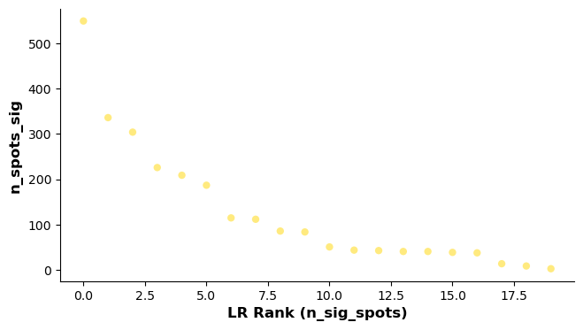
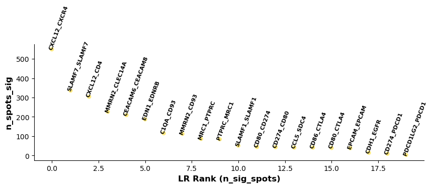
[33]:
# Showing the rankings of the LR from a global and local perspective.
# Ranking based on number of significant hotspots.
st.pl.lr_summary(grid, n_top=500)
st.pl.lr_summary(grid, n_top=50, figsize=(10,3))
[34]:
### Can adjust significance thresholds.
st.tl.cci.adj_pvals(grid, correct_axis='spot',
                   pval_adj_cutoff=0.05, adj_method='fdr_bh')
Updated adata.uns[lr_summary]
Updated adata.obsm[lr_scores]
Updated adata.obsm[lr_sig_scores]
Updated adata.obsm[p_vals]
Updated adata.obsm[p_adjs]
Updated adata.obsm[-log10(p_adjs)]
Downstream visualisations from LR analsyis
For more downstream visualisations, please see the stLearn CCI tutorial:
https://stlearn.readthedocs.io/en/latest/tutorials/stLearn-CCI.html
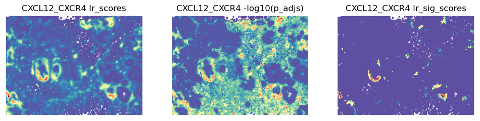
[35]:
best_lr = grid.uns['lr_summary'].index.values[0] # Just choosing one of the top from lr_summary
[36]:
stats = ['lr_scores', '-log10(p_adjs)', 'lr_sig_scores']
fig, axes = plt.subplots(ncols=len(stats), figsize=(12,6))
for i, stat in enumerate(stats):
    st.pl.lr_result_plot(grid, use_result=stat, use_lr=best_lr, show_color_bar=False, ax=axes[i])
    axes[i].set_title(f'{best_lr} {stat}')
Predicting Significant Cell-Cell Interactions
For this analysis, we are using within-spot mode, with the deconvolution information which is stored in grid.uns, as automatically determined by st.tl.cci.grid. The permutation is performed to permute the cell proportions associated with each spot, to determine spots located in LR hotspots that have certain cell types over-represented.
[41]:
grid
[41]:
AnnData object with n_obs × n_vars = 14521 × 313
    obs: 'imagecol', 'imagerow', 'n_cells', 'louvain', 'group'
    uns: 'spatial', 'louvain', 'louvain_colors', 'grid_counts', 'grid_xedges', 'grid_yedges', 'lrfeatures', 'lr_summary'
    obsm: 'spatial', 'spot_neighbours', 'spot_neigh_bcs', 'lr_scores', 'p_vals', 'p_adjs', '-log10(p_adjs)', 'lr_sig_scores'
[42]:
st.tl.cci.run_cci(grid, 'louvain', # Spot cell information either in data.obs or data.uns
                  min_spots=2, # Minimum number of spots for LR to be tested.
                  spot_mixtures=True, # If True will use the deconvolution data,
                                      # so spots can have multiple cell types if score>cell_prop_cutoff
                  cell_prop_cutoff=0.1, # Spot considered to have cell type if score>0.1
                  sig_spots=True, # Only consider neighbourhoods of spots which had significant LR scores.
                  n_perms=100, # Permutations of cell information to get background, recommend ~1000
                  n_cpus=None,
                 )
Getting cached neighbourhood information...
Getting information for CCI counting...
Counting celltype-celltype interactions per LR and permutating 100 times.: 100%|██████████████████ [ time left: 00:00 ]
Significant counts of cci_rank interactions for all LR pairs in data.uns[lr_cci_louvain]
Significant counts of cci_rank interactions for each LR pair stored in dictionary data.uns[per_lr_cci_louvain]
[49]:
st.tl.cci.run_cci(grid, 'louvain', # Spot cell information either in data.obs or data.uns
                  min_spots=2, # Minimum number of spots for LR to be tested.
                  spot_mixtures=True, # If True will use the deconvolution data,
                                      # so spots can have multiple cell types if score>cell_prop_cutoff
                  cell_prop_cutoff=0.1, # Spot considered to have cell type if score>0.1
                  sig_spots=True, # Only consider neighbourhoods of spots which had significant LR scores.
                  n_perms=100, # Permutations of cell information to get background, recommend ~1000
                  n_cpus=10,
                 )
Getting cached neighbourhood information...
Getting information for CCI counting...
Counting celltype-celltype interactions per LR and permutating 100 times.: 100%|███████████████████████████████████████████████████████████████████████████████████████████████████████ [ time left: 00:00 ]
Significant counts of cci_rank interactions for all LR pairs in data.uns[lr_cci_louvain]
Significant counts of cci_rank interactions for each LR pair stored in dictionary data.uns[per_lr_cci_louvain]
Diagnostic: checking for interaction and cell type frequency correlation
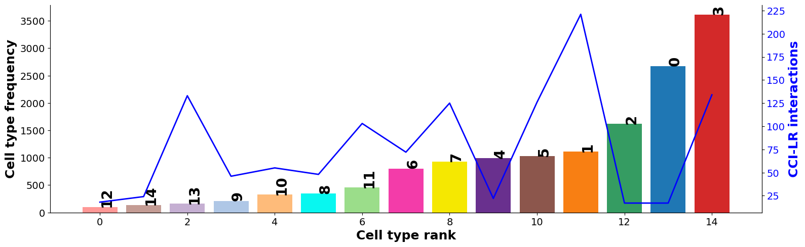
Should be little to no correlation; indicating the permutation has adequately controlled for cell type frequency.
[43]:
st.pl.cci_check(grid, 'louvain', figsize=(16,5))
CCI Visualisations
CCI Network Plot
[44]:
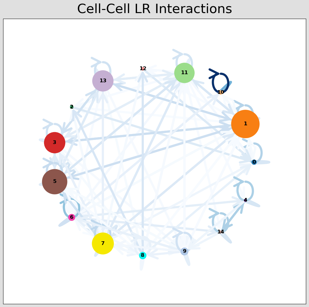
# Visualising the no. of interactions between cell types across all LR pairs #
pos_1 = st.pl.ccinet_plot(grid, 'louvain', return_pos=True, min_counts=30)
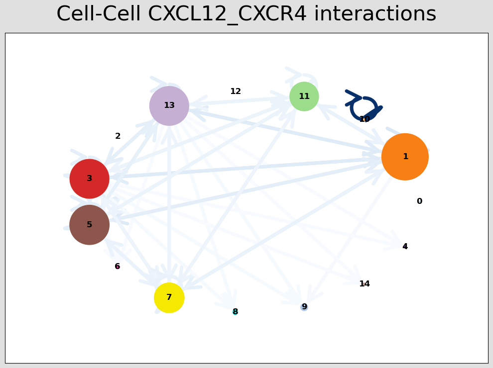
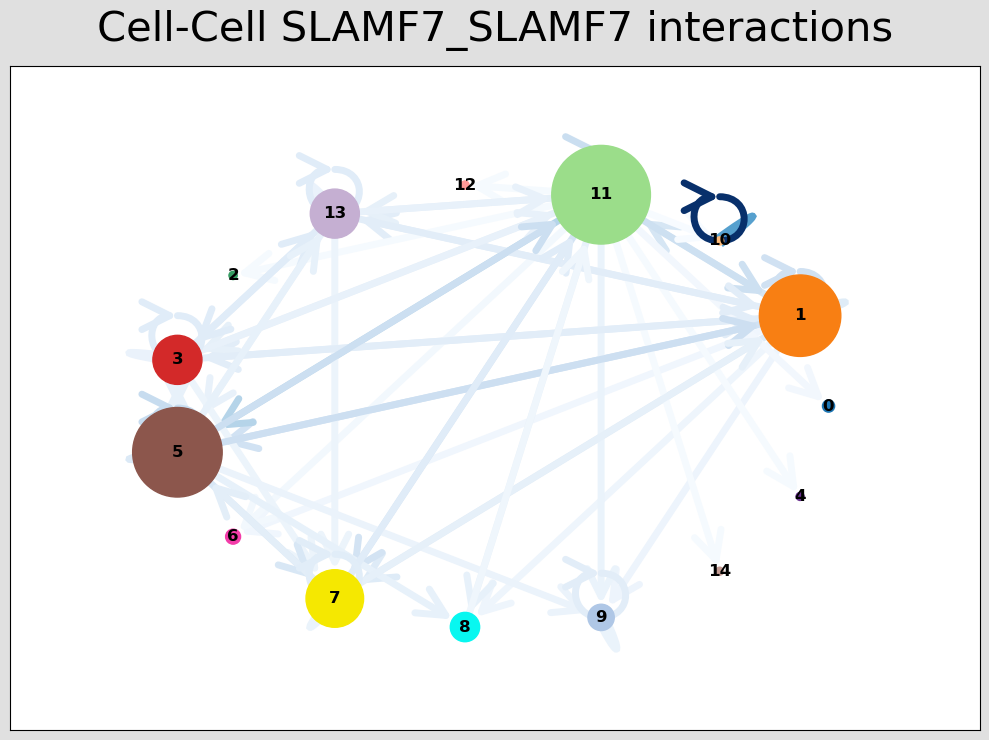
# Just examining the cell type interactions between selected pairs #
lrs = grid.uns['lr_summary'].index.values[0:3]
for best_lr in lrs[0:2]:
st.pl.ccinet_plot(grid, 'louvain', best_lr, min_counts=2,
figsize=(10,7.5), pos=pos_1,
)
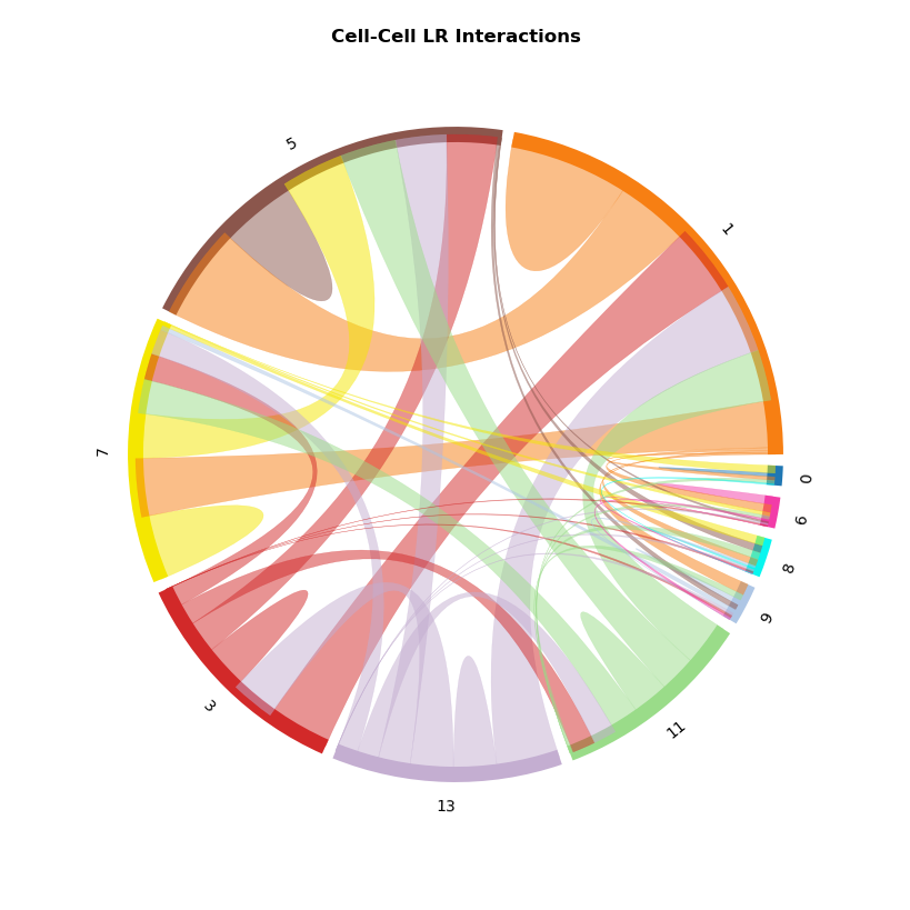
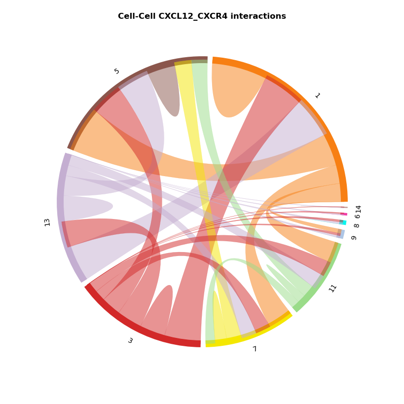
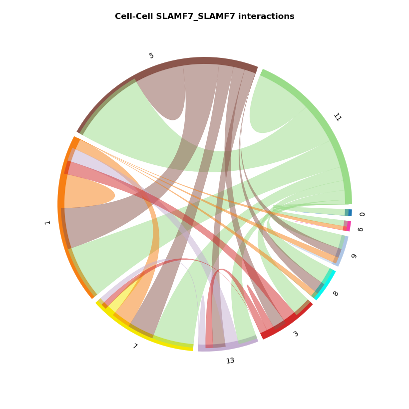
CCI Chord Plot
[45]:
st.pl.lr_chord_plot(grid, 'louvain')

for lr in lrs[0:2]:
    st.pl.lr_chord_plot(grid, 'louvain', lr)
For additional visualisations and visualisation tips, please see:
https://stlearn.readthedocs.io/en/latest/tutorials/stLearn-CCI.html
Acknowledgement
We would like to thank Soo Hee Lee and 10X Genomics team for their able support, contribution and feedback to this tutorial