Xenium data analysis with spatial trajectories inference

We will go through the tutorial on how to use stLearn to perform clustering (with or without imputation) and spatial trajectories inference with Xenium data from 10X Genomics. The main dataset we are working on is the breast cancer tumor microenvironment. You can download it here: https://www.10xgenomics.com/products/xenium-in-situ/preview-dataset-human-breast

1. Loading library

import stlearn as st
import scanpy as sc
import numpy as np

2. Reading Xenium data

You can download all the data in the 10X Genomics resource webpage. For H&E image, because it was generated separately with the main xenium data, then you need to perform the registration by your self. Here we provide an example of a H&E image which is performed a manual registration by Dr. Soo Hee Lee. You can download it here: Link

adata = st.ReadXenium(feature_cell_matrix_file="Xenium_FFPE_Human_Breast_Cancer_Rep1_cell_feature_matrix.h5",
                     cell_summary_file="Xenium_FFPE_Human_Breast_Cancer_Rep1_cells.csv.gz",
                     library_id="Xenium_FFPE_Human_Breast_Cancer_Rep1",
                     image_path="CS1384_post-CS0_H&E_S1A_RGB-shlee-crop.png",
                     scale=1,
                     spot_diameter_fullres=15 # Recommend
                     )

Added tissue image to the object!

adata

AnnData object with n_obs × n_vars = 167782 × 313
    obs: 'imagecol', 'imagerow'
    var: 'gene_ids', 'feature_types', 'genome'
    uns: 'spatial'
    obsm: 'spatial'

3. Preprocessing

Here, we use scanpy to perform several steps of preprocessing

# Filter genes and cells with at least 10 counts
sc.pp.filter_genes(adata, min_counts=10)
sc.pp.filter_cells(adata,min_counts=10)

# Store the raw data for using PSTS
adata.raw = adata

# Normalization data
sc.pp.normalize_total(adata)

After normalization, we have two options. One is using log transformation or square root transformation (recommend by the 10X team)

# Squareroot normalize transcript counts. We need to deal with sparse matrix of .X
from scipy.sparse import csr_array
adata.X = np.sqrt(adata.X.toarray()) + np.sqrt(adata.X.toarray() + 1)
# If the matrix is small, we don't need to convert to numpy array. I believe, Xenium data is always large
# adata.X = csr_array(np.sqrt(adata.X) + np.sqrt(adata.X + 1))

# If you want to use log transformation, please use:
# st.pp.log1p(adata)

# Run PCA
st.em.run_pca(adata,n_comps=50,random_state=0)

PCA is done! Generated in adata.obsm['X_pca'], adata.uns['pca'] and adata.varm['PCs']

Apply stSME (optional)

stSME is optional as an imputation function. Due to the scope of this tutorial, we will not use it here, but we recommend you run if you have an H&E image in your dataset

# apply stSME to normalise log transformed data
# st.spatial.SME.SME_normalize(adata, use_data="raw")
# adata.X = adata.obsm['raw_SME_normalized']
# st.pp.scale(adata)
# st.em.run_pca(adata,n_comps=50)

# Compute neighborhood graph of cells using the PCA representation
st.pp.neighbors(adata,n_neighbors=25,use_rep='X_pca',random_state=0)

Created k-Nearest-Neighbor graph in adata.uns['neighbors']

3. Clustering

Here we use louvain clustering. You also can use leiden clustering method with scanpy.tl.leiden.

st.tl.clustering.louvain(adata,random_state=0)

Applying Louvain cluster ...
Louvain cluster is done! The labels are stored in adata.obs['louvain']

We can plot the clustering result:

import matplotlib.pyplot as plt
plt.rcParams["figure.figsize"] = (10,10)
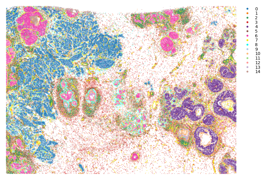
st.pl.cluster_plot(adata,use_label="louvain",image_alpha=0,size=1)

You can crop a region of interest with zoom_coord parameter.

plt.rcParams["figure.figsize"] = (3,3)
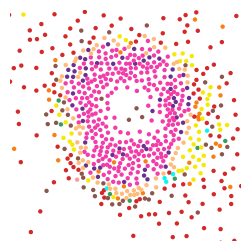
st.pl.cluster_plot(adata,use_label="louvain",
                   image_alpha=0,size=10,
                   zoom_coord=[4000,4400,4700,5100],
                   show_color_bar=False)

4. PSeudo-Time-Space (PSTS) for spatial trajectory analysis

We provide PSTS for spatial trajectory analysis.

The first step is to select the root index. We allow the user to automatically select the index of the cell but still need to input which cluster should be the root cluster in your biological question.

In this tutorial, we focus on the cancer progression from Ductal carcinoma in situ (DCIS) to Invasive ductal carcinoma (IDC). That is why we choose the root cluster 6 as the DCIS cluster.

adata.uns["iroot"] = st.spatial.trajectory.set_root(
    adata,
    use_label="louvain",
    cluster="6",
    use_raw=True
)
adata.uns["iroot"]

104132

For the pseudotime function, we are based on the diffusion pseudotime algorithm to initialize the pseudotime for trajectory at the gene expression level. pseudotimespace_global is the function for incorporating the spatial information to construct the (meta) trajectory in the spatial context.

st.spatial.trajectory.pseudotime(adata,eps=50,use_rep="X_pca",use_label="louvain")

D:\Anaconda3\envs\stlearn\lib\site-packages\anndata\_core\anndata.py:1228: FutureWarning: The `inplace` parameter in pandas.Categorical.reorder_categories is deprecated and will be removed in a future version. Reordering categories will always return a new Categorical object.
  c.reorder_categories(natsorted(c.categories), inplace=True)
... storing 'feature_types' as categorical
D:\Anaconda3\envs\stlearn\lib\site-packages\anndata\_core\anndata.py:1228: FutureWarning: The `inplace` parameter in pandas.Categorical.reorder_categories is deprecated and will be removed in a future version. Reordering categories will always return a new Categorical object.
  c.reorder_categories(natsorted(c.categories), inplace=True)
... storing 'genome' as categorical

All available trajectory paths are stored in adata.uns['available_paths'] with length < 4 nodes

In this dataset, the IDC cluster we are looking for is the one on the edge of ducts. This part is the first layer of invasive cancer cells starting from DCIS. That’s how we choose cluster 10 for the IDC.

st.spatial.trajectory.pseudotimespace_global(adata,use_label="louvain",list_clusters=["6","10"])

Start to construct the trajectory: 6 -> 10

After construct the spatial trajectories from DCIS to IDC cluster. We can observe multiple meta-trajectories with sub-clusters which generated by spatial feature. With tree_plot, you can show all of the detail sub-clusters ids.

st.pl.trajectory.tree_plot(adata,figsize=(10,15),ncols=4)

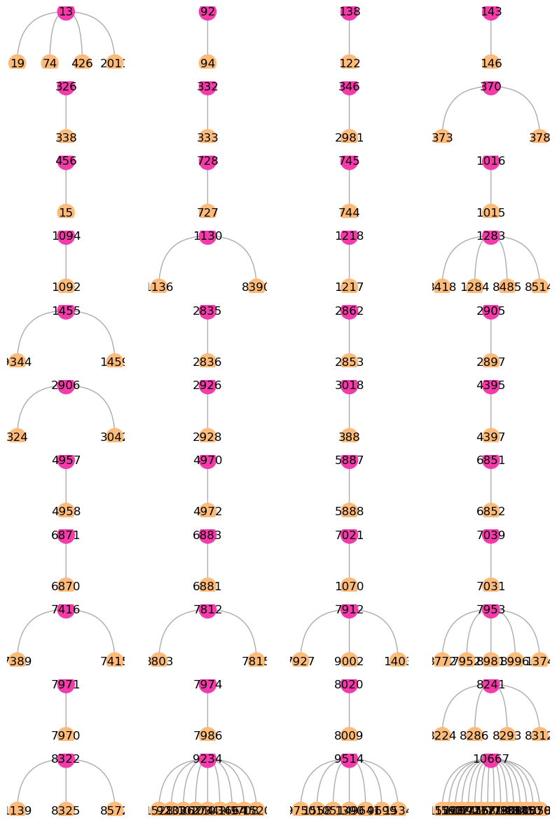
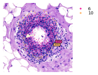
Now, we can crop and discover the transition genes of sub-clusters 1094 -> 1092 meta-trajectory

st.pl.cluster_plot(
    adata,
    use_label="louvain",
    show_trajectories=True,
    list_clusters=["6","10"],
    show_subcluster=True,
    zoom_coord=[4000,4400,4700,5100],
    show_node=False
)

Finding the transition markers of clade_1094

st.spatial.trajectory.detect_transition_markers_clades(adata,clade=1094,use_raw_count=False,cutoff_spearman=0.1)

Detecting the transition markers of clade_1094...
Transition markers result is stored in adata.uns['clade_1094']

Plot the transition markers, red color is down-regulated gene, blue color is up-regulated gene

plt.rcParams["figure.figsize"] = (5,5)
st.pl.trajectory.transition_markers_plot(adata,top_genes=20,trajectory="clade_1094")

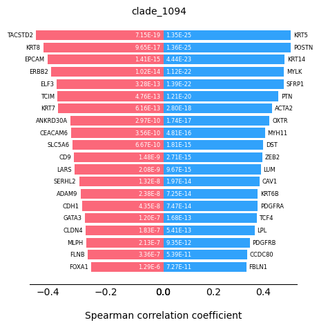
We can observe some keratinocytes family genes here as the progression markers.

Acknowledgement

We would like to thank Soo Hee Lee and 10X Genomics team for their able support, contribution and feedback to this tutorial