Pseudotime Spatial Trajectory Inference¶

In this tutorial, we are using both spatial information and gene expression profile to perform spatial trajectory inference to explore the progression of Ductal Carcinoma in situ (DCIS) - Invasive Ductal Cancer (IDC)

Source: https://www.10xgenomics.com/datasets/human-breast-cancer-block-a-section-1-1-standard-1-1-0

1. Preparation¶

We are trying to keep it focus on spatial trajectory inference then every step from reading data, processing to clustering, we will give the code here to easier for user to use.

Read and preprocess data¶

[1]:

import os
import platform

# Only constrain threads on macOS where BLAS/numba deadlocks are common.
# Must run before any numpy/scanpy import.
if platform.system() == "Darwin":
    os.environ["OPENBLAS_NUM_THREADS"] = "1"
    os.environ["MKL_NUM_THREADS"] = "1"
    os.environ["NUMBA_NUM_THREADS"] = "1"
    n_cpus = 1
else:
    n_cpus = None

[2]:

seed = 0
os.environ['PYTHONHASHSEED'] = str(seed)

import random as random
import stlearn as st
import pathlib as pathlib
import numpy as np

st.settings.set_figure_params(dpi=120)

# Make sure all the seeds are set
np.random.seed(seed)
random.seed(seed)

# Ignore all warnings
import warnings
warnings.filterwarnings("ignore")

[3]:

# Read raw data
st.settings.datasetdir = pathlib.Path.cwd().parent / "data"
data = st.datasets.visium_sge(sample_id="V1_Breast_Cancer_Block_A_Section_1")
data = st.convert_scanpy(data)

[4]:

# Save raw_count
data.layers["raw_count"] = data.X
# Preprocessing
st.pp.filter_genes(data, min_cells=3)
st.pp.normalize_total(data)
st.pp.log1p(data)
# Keep raw data
data.raw = data
st.pp.scale(data)

Normalization step is finished in adata.X
Log transformation step is finished in adata.X
Scale step is finished in adata.X

Clustering data¶

[5]:

# Run PCA
st.em.run_pca(data, n_comps=50, random_state=seed)
# Tiling image
st.pp.tiling(data, out_path="tiling", crop_size=40, quality=95)
# Using Deep Learning to extract feature
st.pp.extract_feature(data)

PCA is done! Generated in adata.obsm['X_pca'], adata.uns['pca'] and adata.varm['PCs']

Tiling image: 100%|████████████████████████████████████████████████████████████████████████████████████████████████████████████████████████████████████████████████████████████████████████████ [ time left: 00:00 ]
Extract feature:  97%|████████████████████████████████████████████████████████████████████████████████████████████████████████████████████████████████████████████████████████████████████▋     [ time left: 00:00 ]

The morphology feature is added to adata.obsm['X_morphology']!

[6]:

# Apply stSME spatial-PCA option
st.spatial.morphology.adjust(data, use_data="X_pca", radius=50, method="mean")

Adjusting data: 100%|██████████████████████████████████████████████████████████████████████████████████████████████████████████████████████████████████████████████████████████████████████████ [ time left: 00:00 ]

The data adjusted by morphology is added to adata.obsm['X_pca_morphology']

[7]:

st.pp.neighbors(data, n_neighbors=25, use_rep='X_pca_morphology', random_state=seed)
st.tl.clustering.leiden(data, resolution=0.8, random_state=seed)
st.pl.cluster_plot(data, use_label="leiden", image_alpha=1, size=7, bbox_to_anchor=(1.3, 1))

Created k-Nearest-Neighbor graph in adata.uns['neighbors']
Applying Leiden cluster ...
Leiden cluster is done! The labels are stored in adata.obs['leiden']

[7]:

AnnData object with n_obs × n_vars = 3798 × 22240
    obs: 'in_tissue', 'array_row', 'array_col', 'imagecol', 'imagerow', 'tile_path', 'leiden'
    var: 'gene_ids', 'feature_types', 'genome', 'n_cells', 'mean', 'std'
    uns: 'spatial', 'log1p', 'pca', 'neighbors', 'leiden', 'leiden_colors'
    obsm: 'spatial', 'X_pca', 'X_tile_feature', 'X_morphology', 'X_pca_morphology'
    varm: 'PCs'
    layers: 'raw_count'
    obsp: 'distances', 'connectivities'

../_images/tutorials_pseudotime_space_12_2.png

[8]:

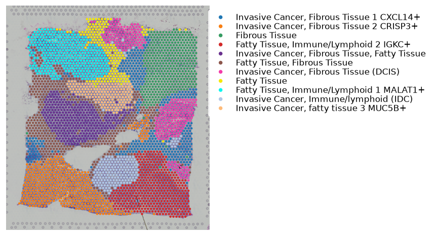
st.add.annotation(data, label_list=['Invasive Cancer, Fibrous Tissue 1 CXCL14+',
                                    'Invasive Cancer, Fibrous Tissue 2 CRISP3+',
                                    'Fibrous Tissue',
                                    'Fatty Tissue, Immune/Lymphoid 2 IGKC+',
                                    'Invasive Cancer, Fibrous Tissue, Fatty Tissue',
                                    'Fatty Tissue, Fibrous Tissue',
                                    'Invasive Cancer, Fibrous Tissue (DCIS)',
                                    'Fatty Tissue',
                                    'Fatty Tissue, Immune/Lymphoid 1 MALAT1+',
                                    'Invasive Cancer, Immune/lymphoid (IDC)',
                                    'Invasive Cancer, fatty tissue 3 MUC5B+',
                                    ],
                  use_label="leiden")
st.pl.cluster_plot(data, use_label="leiden_anno", image_alpha=1, size=7, bbox_to_anchor=(2.1, 1))

The annotation is added to adata.obs['leiden_anno']

[8]:

AnnData object with n_obs × n_vars = 3798 × 22240
    obs: 'in_tissue', 'array_row', 'array_col', 'imagecol', 'imagerow', 'tile_path', 'leiden', 'leiden_anno'
    var: 'gene_ids', 'feature_types', 'genome', 'n_cells', 'mean', 'std'
    uns: 'spatial', 'log1p', 'pca', 'neighbors', 'leiden', 'leiden_colors', 'leiden_anno_colors'
    obsm: 'spatial', 'X_pca', 'X_tile_feature', 'X_morphology', 'X_pca_morphology'
    varm: 'PCs'
    layers: 'raw_count'
    obsp: 'distances', 'connectivities'

../_images/tutorials_pseudotime_space_13_2.png

2. Spatial trajectory inference¶

Choosing root¶

3733 is the index of the spot that we chose as root. It in the DCIS cluster (6). We recommend the root spot should be in the end/begin of a cluster in UMAP space. You can find min/max point of a cluster in UMAP as root.

[9]:

data.uns["iroot"] = st.spatial.trajectory.set_root(data, use_label="leiden", cluster="6", use_raw=True)
st.spatial.trajectory.pseudotime(data, eps=50, use_rep="X_pca", use_label="leiden", threshold_spots=4)

All available trajectory paths are stored in adata.uns['available_paths'] with length < 4 nodes

Spatial trajectory inference - global level¶

We run the global level of pseudo-time-space (PSTS) method to reconstruct the spatial trajectory between cluster 6 (DCIS) and 9 (lesions IDC)

[10]:

st.spatial.trajectory.pseudotimespace_global(data, use_label="leiden", list_clusters=["6", "9"])

Start to construct the trajectory: 6 -> 9

[10]:

AnnData object with n_obs × n_vars = 3798 × 22240
    obs: 'in_tissue', 'array_row', 'array_col', 'imagecol', 'imagerow', 'tile_path', 'leiden', 'leiden_anno', 'sub_cluster_labels', 'dpt_pseudotime'
    var: 'gene_ids', 'feature_types', 'genome', 'n_cells', 'mean', 'std'
    uns: 'spatial', 'log1p', 'pca', 'neighbors', 'leiden', 'leiden_colors', 'leiden_anno_colors', 'iroot', 'leiden_index_dict', 'paga', 'leiden_sizes', 'diffmap_evals', 'threshold_spots', 'split_node', 'global_graph', 'centroid_dict', 'available_paths', 'PTS_graph'
    obsm: 'spatial', 'X_pca', 'X_tile_feature', 'X_morphology', 'X_pca_morphology', 'X_diffmap'
    varm: 'PCs'
    layers: 'raw_count'
    obsp: 'distances', 'connectivities'

[11]:

st.pl.cluster_plot(data, use_label="leiden", show_trajectories=True, list_clusters=["6", "9"], show_subcluster=True)

[11]:

AnnData object with n_obs × n_vars = 3798 × 22240
    obs: 'in_tissue', 'array_row', 'array_col', 'imagecol', 'imagerow', 'tile_path', 'leiden', 'leiden_anno', 'sub_cluster_labels', 'dpt_pseudotime'
    var: 'gene_ids', 'feature_types', 'genome', 'n_cells', 'mean', 'std'
    uns: 'spatial', 'log1p', 'pca', 'neighbors', 'leiden', 'leiden_colors', 'leiden_anno_colors', 'iroot', 'leiden_index_dict', 'paga', 'leiden_sizes', 'diffmap_evals', 'threshold_spots', 'split_node', 'global_graph', 'centroid_dict', 'available_paths', 'PTS_graph'
    obsm: 'spatial', 'X_pca', 'X_tile_feature', 'X_morphology', 'X_pca_morphology', 'X_diffmap'
    varm: 'PCs'
    layers: 'raw_count'
    obsp: 'distances', 'connectivities'

../_images/tutorials_pseudotime_space_19_1.png

[12]:

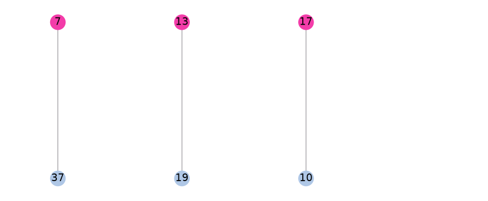
st.pl.trajectory.tree_plot(data, use_label="leiden", show_all=True)

../_images/tutorials_pseudotime_space_20_0.png

[12]:

AnnData object with n_obs × n_vars = 3798 × 22240
    obs: 'in_tissue', 'array_row', 'array_col', 'imagecol', 'imagerow', 'tile_path', 'leiden', 'leiden_anno', 'sub_cluster_labels', 'dpt_pseudotime'
    var: 'gene_ids', 'feature_types', 'genome', 'n_cells', 'mean', 'std'
    uns: 'spatial', 'log1p', 'pca', 'neighbors', 'leiden', 'leiden_colors', 'leiden_anno_colors', 'iroot', 'leiden_index_dict', 'paga', 'leiden_sizes', 'diffmap_evals', 'threshold_spots', 'split_node', 'global_graph', 'centroid_dict', 'available_paths', 'PTS_graph'
    obsm: 'spatial', 'X_pca', 'X_tile_feature', 'X_morphology', 'X_pca_morphology', 'X_diffmap'
    varm: 'PCs'
    layers: 'raw_count'
    obsp: 'distances', 'connectivities'

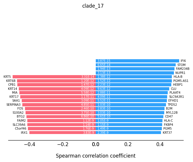
Transition markers detection¶

Based on the spatial trajectory/tree plot, we can see clades are started from sub-cluster 7, 13 and 17. Then we run the function to detect the highly correlated genes with the PSTS values.

[13]:

st.spatial.trajectory.detect_transition_markers_clades(data, clade=7, use_raw_count=False, cutoff_spearman=0.4)

Detecting the transition markers of clade_7...
Transition markers result is stored in adata.uns['clade_7']

[14]:

st.spatial.trajectory.detect_transition_markers_clades(data, clade=13, use_raw_count=False, cutoff_spearman=0.4)

Detecting the transition markers of clade_13...
Transition markers result is stored in adata.uns['clade_13']

[15]:

st.spatial.trajectory.detect_transition_markers_clades(data, clade=17, use_raw_count=False, cutoff_spearman=0.4)

Detecting the transition markers of clade_17...
Transition markers result is stored in adata.uns['clade_17']

[16]:

data.uns['clade_7'] = data.uns['clade_7'][data.uns['clade_7']['gene'].map(lambda x: "RPL" not in x)]
data.uns['clade_13'] = data.uns['clade_13'][data.uns['clade_13']['gene'].map(lambda x: "RPL" not in x)]
data.uns['clade_17'] = data.uns['clade_17'][data.uns['clade_17']['gene'].map(lambda x: "RPL" not in x)]
data.uns['clade_7'] = data.uns['clade_7'][data.uns['clade_7']['gene'].map(lambda x: "RPS" not in x)]
data.uns['clade_13'] = data.uns['clade_13'][data.uns['clade_13']['gene'].map(lambda x: "RPS" not in x)]
data.uns['clade_17'] = data.uns['clade_17'][data.uns['clade_17']['gene'].map(lambda x: "RPS" not in x)]

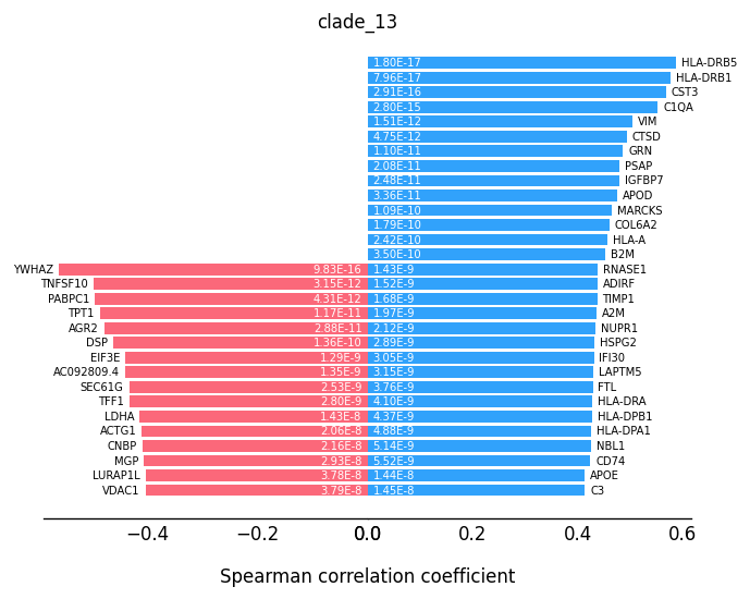
For the transition markers plot, genes from left side (red) are negatively correlated with the spatial trajectory and genes from right side (blue) are positively correlated with the spatial trajectory.

[17]:

st.pl.trajectory.transition_markers_plot(data, top_genes=30, trajectory="clade_7")

../_images/tutorials_pseudotime_space_27_0.png

[17]:

AnnData object with n_obs × n_vars = 3798 × 22240
    obs: 'in_tissue', 'array_row', 'array_col', 'imagecol', 'imagerow', 'tile_path', 'leiden', 'leiden_anno', 'sub_cluster_labels', 'dpt_pseudotime'
    var: 'gene_ids', 'feature_types', 'genome', 'n_cells', 'mean', 'std'
    uns: 'spatial', 'log1p', 'pca', 'neighbors', 'leiden', 'leiden_colors', 'leiden_anno_colors', 'iroot', 'leiden_index_dict', 'paga', 'leiden_sizes', 'diffmap_evals', 'threshold_spots', 'split_node', 'global_graph', 'centroid_dict', 'available_paths', 'PTS_graph', 'clade_7', 'clade_13', 'clade_17'
    obsm: 'spatial', 'X_pca', 'X_tile_feature', 'X_morphology', 'X_pca_morphology', 'X_diffmap'
    varm: 'PCs'
    layers: 'raw_count'
    obsp: 'distances', 'connectivities'

[18]:

st.pl.trajectory.transition_markers_plot(data, top_genes=30, trajectory="clade_13")

../_images/tutorials_pseudotime_space_28_0.png

[18]:

AnnData object with n_obs × n_vars = 3798 × 22240
    obs: 'in_tissue', 'array_row', 'array_col', 'imagecol', 'imagerow', 'tile_path', 'leiden', 'leiden_anno', 'sub_cluster_labels', 'dpt_pseudotime'
    var: 'gene_ids', 'feature_types', 'genome', 'n_cells', 'mean', 'std'
    uns: 'spatial', 'log1p', 'pca', 'neighbors', 'leiden', 'leiden_colors', 'leiden_anno_colors', 'iroot', 'leiden_index_dict', 'paga', 'leiden_sizes', 'diffmap_evals', 'threshold_spots', 'split_node', 'global_graph', 'centroid_dict', 'available_paths', 'PTS_graph', 'clade_7', 'clade_13', 'clade_17'
    obsm: 'spatial', 'X_pca', 'X_tile_feature', 'X_morphology', 'X_pca_morphology', 'X_diffmap'
    varm: 'PCs'
    layers: 'raw_count'
    obsp: 'distances', 'connectivities'

[19]:

st.pl.trajectory.transition_markers_plot(data, top_genes=30, trajectory="clade_17")

../_images/tutorials_pseudotime_space_29_0.png

[19]:

AnnData object with n_obs × n_vars = 3798 × 22240
    obs: 'in_tissue', 'array_row', 'array_col', 'imagecol', 'imagerow', 'tile_path', 'leiden', 'leiden_anno', 'sub_cluster_labels', 'dpt_pseudotime'
    var: 'gene_ids', 'feature_types', 'genome', 'n_cells', 'mean', 'std'
    uns: 'spatial', 'log1p', 'pca', 'neighbors', 'leiden', 'leiden_colors', 'leiden_anno_colors', 'iroot', 'leiden_index_dict', 'paga', 'leiden_sizes', 'diffmap_evals', 'threshold_spots', 'split_node', 'global_graph', 'centroid_dict', 'available_paths', 'PTS_graph', 'clade_7', 'clade_13', 'clade_17'
    obsm: 'spatial', 'X_pca', 'X_tile_feature', 'X_morphology', 'X_pca_morphology', 'X_diffmap'
    varm: 'PCs'
    layers: 'raw_count'
    obsp: 'distances', 'connectivities'

[20]:

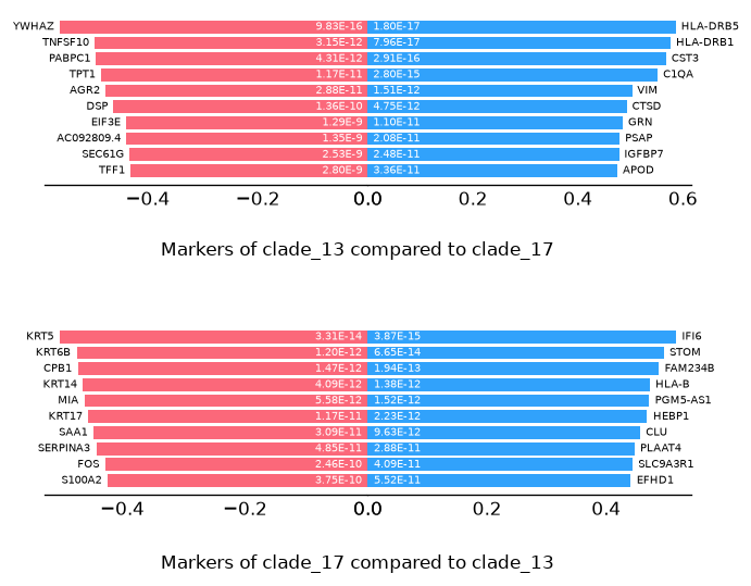
st.spatial.trajectory.compare_transitions(data, trajectories=["clade_13", "clade_17"])

The result of comparison between clade_13 and clade_17 stored in 'adata.uns['compare_result']'

[21]:

st.pl.trajectory.de_transition_plot(data)

../_images/tutorials_pseudotime_space_31_0.png

[21]:

AnnData object with n_obs × n_vars = 3798 × 22240
    obs: 'in_tissue', 'array_row', 'array_col', 'imagecol', 'imagerow', 'tile_path', 'leiden', 'leiden_anno', 'sub_cluster_labels', 'dpt_pseudotime'
    var: 'gene_ids', 'feature_types', 'genome', 'n_cells', 'mean', 'std'
    uns: 'spatial', 'log1p', 'pca', 'neighbors', 'leiden', 'leiden_colors', 'leiden_anno_colors', 'iroot', 'leiden_index_dict', 'paga', 'leiden_sizes', 'diffmap_evals', 'threshold_spots', 'split_node', 'global_graph', 'centroid_dict', 'available_paths', 'PTS_graph', 'clade_7', 'clade_13', 'clade_17', 'compare_result'
    obsm: 'spatial', 'X_pca', 'X_tile_feature', 'X_morphology', 'X_pca_morphology', 'X_diffmap'
    varm: 'PCs'
    layers: 'raw_count'
    obsp: 'distances', 'connectivities'

We also provide a function to compare the transition markers between two clades.