stSME Clustering¶

stSME is a novel normalisation method implemented in stLearn software.

It’s designed for spatial transcriptomics data and utilised tissue Spatial location, Morphology, , and gene Expression.

This tutorial demonstrates how to use stLearn to perform stSME clustering for spatial transcriptomics data

In this tutorial we first focus on Mouse Brain (Coronal) Visium dataset from 10x genomics website.

Mouse Brain (Coronal)¶

1. Preparation¶

[1]:

import os
import platform

# Only constrain threads on macOS where BLAS/numba deadlocks are common.
# Must run before any numpy/scanpy import.
if platform.system() == "Darwin":
    os.environ["OPENBLAS_NUM_THREADS"] = "1"
    os.environ["MKL_NUM_THREADS"] = "1"
    os.environ["NUMBA_NUM_THREADS"] = "1"
    n_cpus = 1
else:
    n_cpus = None

[2]:

import scanpy as sc
import stlearn as st
import pathlib
import numpy as np
import random
from threadpoolctl import threadpool_limits

st.settings.set_figure_params(dpi=120)

# Make sure all the seeds are set
seed = 0
np.random.seed(seed)
random.seed(seed)
os.environ['PYTHONHASHSEED'] = str(seed)

# Ignore all warnings
import warnings
warnings.filterwarnings("ignore")

[3]:

st.settings.datasetdir =  pathlib.Path.cwd().parent / "data"

[4]:

mouse_brain_coronal = sc.datasets.visium_sge(sample_id="V1_Adult_Mouse_Brain")
mouse_brain_coronal = st.convert_scanpy(mouse_brain_coronal)

[5]:

# pre-processing for gene count table
st.pp.filter_genes(mouse_brain_coronal, min_cells=1)
st.pp.normalize_total(mouse_brain_coronal)
st.pp.log1p(mouse_brain_coronal)

Normalization step is finished in adata.X
Log transformation step is finished in adata.X

[6]:

# pre-processing for spot image
st.pp.tiling(mouse_brain_coronal, out_path="tiling")

# this step uses deep learning model to extract high-level features from tile images
# may need few minutes to be completed
st.pp.extract_feature(mouse_brain_coronal, verbose=False)

Tiling image: 100%|████████████████████████████████████████████████████████████████████████████████████████████████████████████████████████████████████████████████████████████████████████████ [ time left: 00:00 ]
Extract feature: 100%|████████████████████████████████████████████████████████████████████████████████████████████████████████████████████████████████████████████████████████████████████████▉ [ time left: 00:00 ]

The morphology feature is added to adata.obsm['X_morphology']!

2. run stSME clustering¶

[7]:

# run PCA for gene expression data
st.em.run_pca(mouse_brain_coronal, n_comps=50)

PCA is done! Generated in adata.obsm['X_pca'], adata.uns['pca'] and adata.varm['PCs']

[8]:

mouse_brain_coronal_sme = mouse_brain_coronal.copy()
# apply stSME to normalise log transformed data
st.spatial.sme.sme_normalize(mouse_brain_coronal_sme, use_data="raw")
mouse_brain_coronal_sme.X = mouse_brain_coronal_sme.obsm['raw_SME_normalized']
st.pp.scale(mouse_brain_coronal_sme)
st.em.run_pca(mouse_brain_coronal_sme, n_comps=50)

Adjusting data: 100%|██████████████████████████████████████████████████████████████████████████████████████████████████████████████████████████████████████████████████████████████████████████ [ time left: 00:00 ]

The data adjusted by SME is added to adata.obsm['raw_SME_normalized']
Scale step is finished in adata.X
PCA is done! Generated in adata.obsm['X_pca'], adata.uns['pca'] and adata.varm['PCs']

[9]:

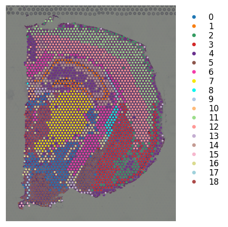
# K-means clustering on stSME normalised PCA
st.tl.clustering.kmeans(mouse_brain_coronal_sme, n_clusters=19, use_data="X_pca", key_added="X_pca_kmeans")
st.pl.cluster_plot(mouse_brain_coronal_sme, use_label="X_pca_kmeans", bbox_to_anchor=(1.3, 1))

Applying Kmeans cluster ...
Kmeans cluster is done! The labels are stored in adata.obs["kmeans"]

[9]:

AnnData object with n_obs × n_vars = 2702 × 21949
    obs: 'in_tissue', 'array_row', 'array_col', 'imagecol', 'imagerow', 'tile_path', 'X_pca_kmeans'
    var: 'gene_ids', 'feature_types', 'genome', 'n_cells', 'mean', 'std'
    uns: 'spatial', 'log1p', 'pca', 'gene_expression_correlation', 'physical_distance', 'morphological_distance', 'weights_matrix_all', 'weights_matrix_pd_gd', 'weights_matrix_pd_md', 'weights_matrix_gd_md', 'X_pca_kmeans_colors'
    obsm: 'spatial', 'X_tile_feature', 'X_morphology', 'X_pca', 'imputed_data', 'top_weights', 'raw_SME_normalized'
    varm: 'PCs'

../_images/tutorials_stsme_clustering_15_2.png

[10]:

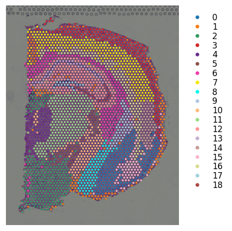
# leiden clustering on stSME normalised data
with threadpool_limits(limits=1, user_api="blas"):
    st.pp.neighbors(mouse_brain_coronal_sme, n_neighbors=17, use_rep='X_pca')
st.tl.clustering.leiden(mouse_brain_coronal_sme, resolution=0.9)
st.pl.cluster_plot(mouse_brain_coronal_sme, use_label="leiden", bbox_to_anchor=(1.3, 1))

Created k-Nearest-Neighbor graph in adata.uns['neighbors']
Applying Leiden cluster ...
Leiden cluster is done! The labels are stored in adata.obs['leiden']

[10]:

AnnData object with n_obs × n_vars = 2702 × 21949
    obs: 'in_tissue', 'array_row', 'array_col', 'imagecol', 'imagerow', 'tile_path', 'X_pca_kmeans', 'leiden'
    var: 'gene_ids', 'feature_types', 'genome', 'n_cells', 'mean', 'std'
    uns: 'spatial', 'log1p', 'pca', 'gene_expression_correlation', 'physical_distance', 'morphological_distance', 'weights_matrix_all', 'weights_matrix_pd_gd', 'weights_matrix_pd_md', 'weights_matrix_gd_md', 'X_pca_kmeans_colors', 'neighbors', 'leiden', 'leiden_colors'
    obsm: 'spatial', 'X_tile_feature', 'X_morphology', 'X_pca', 'imputed_data', 'top_weights', 'raw_SME_normalized'
    varm: 'PCs'
    obsp: 'distances', 'connectivities'

../_images/tutorials_stsme_clustering_16_2.png

we now move to Mouse Brain (Sagittal Posterior) Visium dataset from 10x genomics website.

Mouse Brain (Sagittal Posterior)¶

1. Preparation¶

[11]:

mouse_brain_sagittal = sc.datasets.visium_sge(sample_id="V1_Mouse_Brain_Sagittal_Posterior")
mouse_brain_sagittal = st.convert_scanpy(mouse_brain_sagittal)

[12]:

# pre-processing for gene count table
st.pp.filter_genes(mouse_brain_sagittal, min_cells=1)
st.pp.normalize_total(mouse_brain_sagittal)
st.pp.log1p(mouse_brain_sagittal)
st.pp.scale(mouse_brain_sagittal)

Normalization step is finished in adata.X
Log transformation step is finished in adata.X
Scale step is finished in adata.X

[13]:

# pre-processing for spot image
st.pp.tiling(mouse_brain_sagittal, out_path="tiling")

# this step uses deep learning model to extract high-level features from tile images
# may need few minutes to be completed
st.pp.extract_feature(mouse_brain_sagittal)

Tiling image: 100%|████████████████████████████████████████████████████████████████████████████████████████████████████████████████████████████████████████████████████████████████████████████ [ time left: 00:00 ]
Extract feature:  98%|██████████████████████████████████████████████████████████████████████████████████████████████████████████████████████████████████████████████████████████████████████▎   [ time left: 00:00 ]

The morphology feature is added to adata.obsm['X_morphology']!

2. run stSME clustering¶

[14]:

# run PCA for gene expression data
st.em.run_pca(mouse_brain_sagittal, n_comps=50)

PCA is done! Generated in adata.obsm['X_pca'], adata.uns['pca'] and adata.varm['PCs']

[15]:

mouse_brain_sagittal_sme = mouse_brain_sagittal.copy()
# apply stSME to normalise log transformed data
# with weights from morphological Similarly and physcial distance
st.spatial.sme.sme_normalize(mouse_brain_sagittal_sme, use_data="raw",
                             weights="weights_matrix_pd_md")
mouse_brain_sagittal_sme.X = mouse_brain_sagittal_sme.obsm['raw_SME_normalized']
st.pp.scale(mouse_brain_sagittal_sme)
st.em.run_pca(mouse_brain_sagittal_sme, n_comps=50)

Adjusting data: 100%|██████████████████████████████████████████████████████████████████████████████████████████████████████████████████████████████████████████████████████████████████████████ [ time left: 00:00 ]

The data adjusted by SME is added to adata.obsm['raw_SME_normalized']
Scale step is finished in adata.X
PCA is done! Generated in adata.obsm['X_pca'], adata.uns['pca'] and adata.varm['PCs']

[16]:

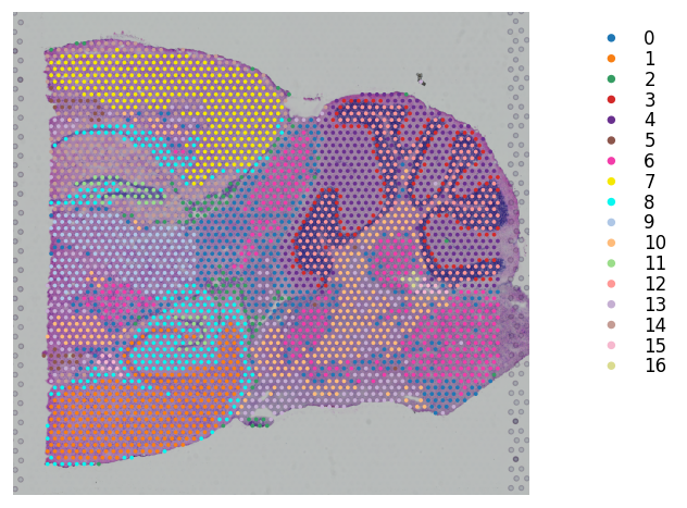
# K-means clustering on stSME normalised PCA
st.tl.clustering.kmeans(mouse_brain_sagittal_sme, n_clusters=17, use_data="X_pca", key_added="X_pca_kmeans")
st.pl.cluster_plot(mouse_brain_sagittal_sme, use_label="X_pca_kmeans", bbox_to_anchor=(1.3, 1))

Applying Kmeans cluster ...
Kmeans cluster is done! The labels are stored in adata.obs["kmeans"]

[16]:

AnnData object with n_obs × n_vars = 3355 × 21363
    obs: 'in_tissue', 'array_row', 'array_col', 'imagecol', 'imagerow', 'tile_path', 'X_pca_kmeans'
    var: 'gene_ids', 'feature_types', 'genome', 'n_cells', 'mean', 'std'
    uns: 'spatial', 'log1p', 'pca', 'gene_expression_correlation', 'physical_distance', 'morphological_distance', 'weights_matrix_all', 'weights_matrix_pd_gd', 'weights_matrix_pd_md', 'weights_matrix_gd_md', 'X_pca_kmeans_colors'
    obsm: 'spatial', 'X_tile_feature', 'X_morphology', 'X_pca', 'imputed_data', 'top_weights', 'raw_SME_normalized'
    varm: 'PCs'

../_images/tutorials_stsme_clustering_26_2.png

[17]:

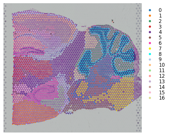
# leiden clustering on stSME normalised data
st.pp.neighbors(mouse_brain_sagittal_sme, n_neighbors=20, use_rep='X_pca')
st.tl.clustering.leiden(mouse_brain_sagittal_sme)
st.pl.cluster_plot(mouse_brain_sagittal_sme, use_label="leiden", bbox_to_anchor=(1.2, 1))

Created k-Nearest-Neighbor graph in adata.uns['neighbors']
Applying Leiden cluster ...
Leiden cluster is done! The labels are stored in adata.obs['leiden']

[17]:

AnnData object with n_obs × n_vars = 3355 × 21363
    obs: 'in_tissue', 'array_row', 'array_col', 'imagecol', 'imagerow', 'tile_path', 'X_pca_kmeans', 'leiden'
    var: 'gene_ids', 'feature_types', 'genome', 'n_cells', 'mean', 'std'
    uns: 'spatial', 'log1p', 'pca', 'gene_expression_correlation', 'physical_distance', 'morphological_distance', 'weights_matrix_all', 'weights_matrix_pd_gd', 'weights_matrix_pd_md', 'weights_matrix_gd_md', 'X_pca_kmeans_colors', 'neighbors', 'leiden', 'leiden_colors'
    obsm: 'spatial', 'X_tile_feature', 'X_morphology', 'X_pca', 'imputed_data', 'top_weights', 'raw_SME_normalized'
    varm: 'PCs'
    obsp: 'distances', 'connectivities'

../_images/tutorials_stsme_clustering_27_2.png

Tutorial by Xiao Tan