stSME Comparison

This tutorial shows the stSME normalization effect between of two scenarios:

• Normal (without stSME)

• stSME applied on raw gene counts

In this tutorial we use Mouse Brain (Coronal) Visium dataset from 10x genomics website.

import os
import platform

# Only constrain threads on macOS where BLAS/numba deadlocks are common.
# Must run before any numpy/scanpy import.
if platform.system() == "Darwin":
    os.environ["OPENBLAS_NUM_THREADS"] = "1"
    os.environ["MKL_NUM_THREADS"] = "1"
    os.environ["NUMBA_NUM_THREADS"] = "1"
    n_cpus = 1
else:
    n_cpus = None

import scanpy as sc
import stlearn as st
import pathlib as pathlib
import numpy as np
import random as random
import os as os

st.settings.set_figure_params(dpi=120)

# Make sure all the seeds are set
seed = 0
np.random.seed(seed)
random.seed(seed)
os.environ['PYTHONHASHSEED'] = str(seed)

# Ignore all warnings
import warnings

warnings.filterwarnings("ignore")

st.settings.datasetdir = pathlib.Path.cwd().parent / "data"

data = sc.datasets.visium_sge(sample_id="V1_Adult_Mouse_Brain")
data = st.convert_scanpy(data)

# pre-processing for gene count table
st.pp.filter_genes(data, min_cells=1)
st.pp.normalize_total(data)
st.pp.log1p(data)

Normalization step is finished in adata.X
Log transformation step is finished in adata.X

# pre-processing for spot image
st.pp.tiling(data, out_path="tiling")

# this step uses deep learning model to extract high-level features from tile images
# may need few minutes to be completed
st.pp.extract_feature(data)

Tiling image: 100%|████████████████████████████████████████████████████████████████████████████████████████████████████████████████████████████████████████████████████████████████████████████ [ time left: 00:00 ]
Extract feature: 100%|████████████████████████████████████████████████████████████████████████████████████████████████████████████████████████████████████████████████████████████████████████▉ [ time left: 00:00 ]

The morphology feature is added to adata.obsm['X_morphology']!

# run PCA for gene expression data
st.em.run_pca(data, n_comps=50)

PCA is done! Generated in adata.obsm['X_pca'], adata.uns['pca'] and adata.varm['PCs']

Normal

data_normal = data.copy()

stSME

data_sme = data.copy()
# apply stSME to normalise log transformed data
st.spatial.sme.sme_normalize(data_sme, use_data="raw")
data_sme.X = data_sme.obsm['raw_SME_normalized']
st.em.run_pca(data_sme, n_comps=50)

Adjusting data: 100%|██████████████████████████████████████████████████████████████████████████████████████████████████████████████████████████████████████████████████████████████████████████ [ time left: 00:00 ]

The data adjusted by SME is added to adata.obsm['raw_SME_normalized']
PCA is done! Generated in adata.obsm['X_pca'], adata.uns['pca'] and adata.varm['PCs']

import matplotlib.pyplot as plt

def plot_comparison(i):
    fig, axes = plt.subplots(1, 2, figsize=(12, 5))

    # Plot into the axes but suppress individual titles
    st.pl.gene_plot(data_normal, gene_symbols=i, size=3, ax=axes[0])
    st.pl.gene_plot(data_sme, gene_symbols=i, size=3, ax=axes[1])

    # Remove individual titles set by the function
    axes[0].set_title("")
    axes[1].set_title("")

    # Set subplot labels and shared title
    axes[0].set_title("Normal", fontsize=12)
    axes[1].set_title("stSME", fontsize=12)
    fig.suptitle(i, fontsize=16, fontweight="bold")

    plt.tight_layout()
    plt.show()

Marker gene for CA3

plot_comparison("Lhfpl1")

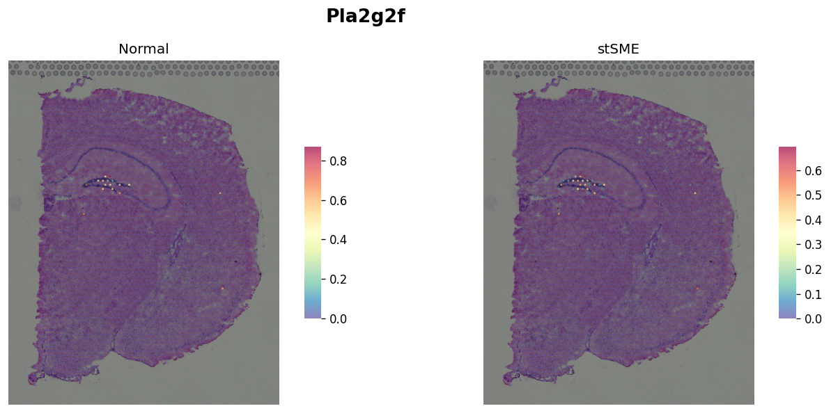
Marker gene for DG

plot_comparison("Pla2g2f")

Tutorial by Xiao Tan